Chapter 4 Examples
4.1 Data subsetting
load_data offers a few tools to help subset data on first load. To get a better sense of how these tools can be put towards practical use, let’s walk through a quick and dirty spatial investigation of poverty and working age population in Chicago.
We start by loading the data dictionary to see what data is available and into what themes they are categorized. This lets us request a subset of the full data set, which minimizes the amount of data in our environment at a time.
# See what data is available
data_dictionary <- load_oeps_dictionary(scale='tract')

# if working in RStudio, we recommend:
# View(data_dictionary)

data_dictionary
Based on the data dictionary, we can see that we have two variables of interest – Age18_64 and PovP. Both variables are available at multiple time periods, and they belong to different themes – social and economic, respectively.
Let’s pull our data using load_oeps. Note how many parameters we provide information for. Geographically, we provide the FIPS code for our desired states (just Illinois) and counties (just Cook), which dramatically cuts down the number of entries retrieved. Additionally, we provide our variables of interests’ themes, lowering the number of rows retrieved.
# Grab the data
cook_county_2010 <- load_oeps(
  scale='tract',
  year='2010',
  themes=c('social', 'economic'),
  states='17',
  counties='031',
  geometry=T)

# Preview what we got
head(data.frame(cook_county_2010))
We can then immediately map our data. We opt to use tmap in this example, but ggplot2 also has mapping functionality for users more familiar with the library.
library(tmap)

tm_shape(cook_county_2010) +
  tm_fill(c('Age18_64', 'PovP'),
          title = c('Working Age', 'Poverty\nPercentage'),
          style = c('sd', 'sd'),
          palette = 'BrBG') +
  tm_layout(legend.position = c('left', 'bottom'), frame=FALSE)
#>
#> ── tmap v3 code detected ───────────────────────────────────────────────────────
#> [v3->v4] `tm_fill()`: instead of `style = "sd"`, use fill.scale =
#> `tm_scale_intervals()`.
#> ℹ Migrate the argument(s) 'style', 'palette' (rename to 'values') to
#>   'tm_scale_intervals(<HERE>)'
#> For small multiples, specify a 'tm_scale_' for each multiple, and put them in a
#> list: 'fill'.scale = list(<scale1>, <scale2>, ...)'
#> [v3->v4] `tm_fill()`: migrate the argument(s) related to the legend of the
#> visual variable `fill` namely 'title' to 'fill.legend = tm_legend(<HERE>)'
#> [cols4all] color palettes: use palettes from the R package cols4all. Run
#> `cols4all::c4a_gui()` to explore them. The old palette name "BrBG" is named
#> "brewer.br_bg"
#> Multiple palettes called "br_bg" found: "brewer.br_bg", "matplotlib.br_bg". The first one, "brewer.br_bg", is returned.
#>
#> Multiple palettes called "br_bg" found: "brewer.br_bg", "matplotlib.br_bg". The first one, "brewer.br_bg", is returned.
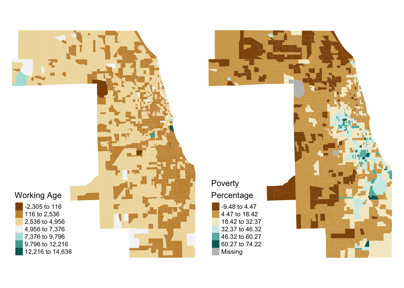
Based on the above, we observe that fewer working age individuals correlates roughly with higher poverty rates within the southern and western sides of Chicago, with this trend breaking down in northern suburbs.
Chicagoland continues a little bit into northeastern Indiana; maybe the rough correlation is present there as well? To check, we can pass a list of county GEOIDS to the counties parameter of load_oeps. Note that these GEOIDS must consist of the state FIPS and county FIPS, as they would otherwise fail to uniquely identify our two counties.
# Grab the data
chicago_metro_2010 <- load_oeps(
  scale='tract',
  year='2010',
  theme=c('social', 'economic'),
  counties=c('17031', '18089'),
  geometry=T)

# Preview what we got
head(data.frame(cook_county_2010))
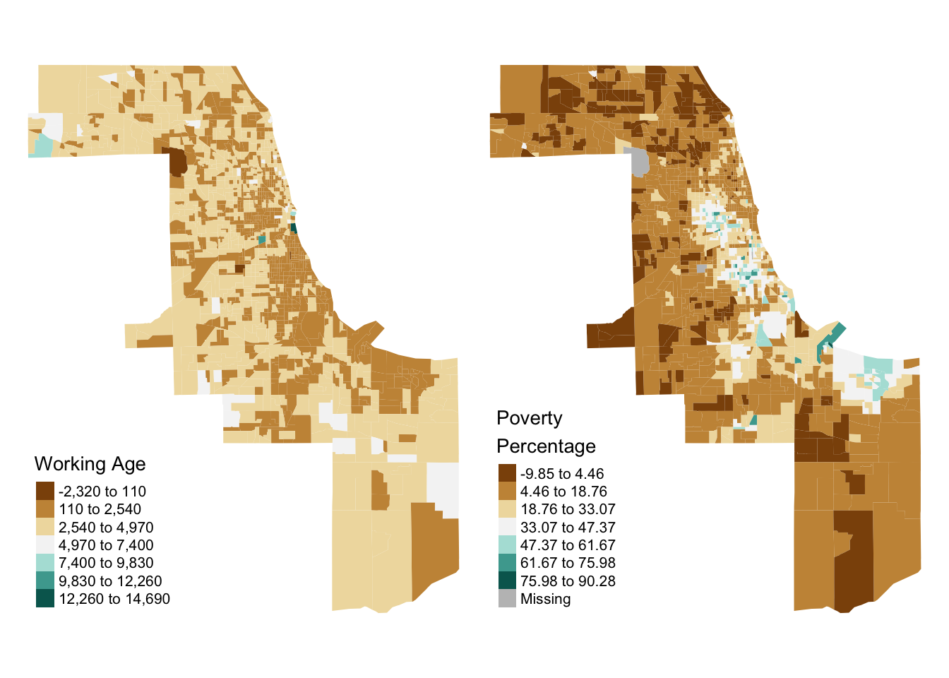
We can once again map the resultant data, and find that the rough correlation between lower working age population totals and higher poverty in more densely populated, coastal areas seems to hold for the broader Chicagoland area.
library(tmap)
tm_shape(chicago_metro_2010) +
  tm_fill(c('Age18_64', 'PovP'),
          title = c('Working Age', 'Poverty\nPercentage'),
          style = c('sd', 'sd'),
          palette = 'BrBG') +
  tm_layout(legend.position = c('left', 'bottom'), frame=FALSE)
#>
#> ── tmap v3 code detected ───────────────────────────────────────────────────────
#> [v3->v4] `tm_fill()`: instead of `style = "sd"`, use fill.scale =
#> `tm_scale_intervals()`.
#> ℹ Migrate the argument(s) 'style', 'palette' (rename to 'values') to
#>   'tm_scale_intervals(<HERE>)'
#> For small multiples, specify a 'tm_scale_' for each multiple, and put them in a
#> list: 'fill'.scale = list(<scale1>, <scale2>, ...)'
#> [v3->v4] `tm_fill()`: migrate the argument(s) related to the legend of the
#> visual variable `fill` namely 'title' to 'fill.legend = tm_legend(<HERE>)'
#> [cols4all] color palettes: use palettes from the R package cols4all. Run
#> `cols4all::c4a_gui()` to explore them. The old palette name "BrBG" is named
#> "brewer.br_bg"
#> Multiple palettes called "br_bg" found: "brewer.br_bg", "matplotlib.br_bg". The first one, "brewer.br_bg", is returned.
#>
#> Multiple palettes called "br_bg" found: "brewer.br_bg", "matplotlib.br_bg". The first one, "brewer.br_bg", is returned.
4.2 Longitudinal analysis
The oepsData package also enables easier longitudinal analysis. Continuing our above example, we might be interested in the change in percent poverty over time throughout Chicagoland. To check, let’s compare 2000 data to 2010 data.
We start by grabbing data from 2000:
# get new data
chicago_metro_2000 <- load_oeps(
  scale='tract',
  year='2000',
  theme=c('social', 'economic'),
  counties=c('17031', '18089'),
  geometry=F)
Because variables have the same column name in every year, chicago_metro_2000 and chicago_metro_2010 have columns with the same names. To fix this, we need to select and rename som eof our columns; there are a wide variety of possible approaches to this problem, but we opt to use dplyr to select and rename our columns of interest.
# rename data columns
chicago_metro_2000 <- dplyr::select(chicago_metro_2000, "HEROP_ID", "PovP2000"="PovP")
chicago_metro_2010 <- dplyr::select(chicago_metro_2010, "HEROP_ID", "PovP2010"="PovP")
We can then merge the dataframes. Two merge keys are provided with oepsData: a HEROP specific merge-key called HEROP_ID and the more common GEOID. We recommend merging on HEROP_ID when merging HEROP data, and reserving GEOID for compatability with outside datasets.
# we changed the name of our merge keys earlier
# so we resolve that here.
chicago_metro_longitudinal <- merge(chicago_metro_2010, chicago_metro_2000,
                                    by.x='HEROP_ID', by.y='HEROP_ID')
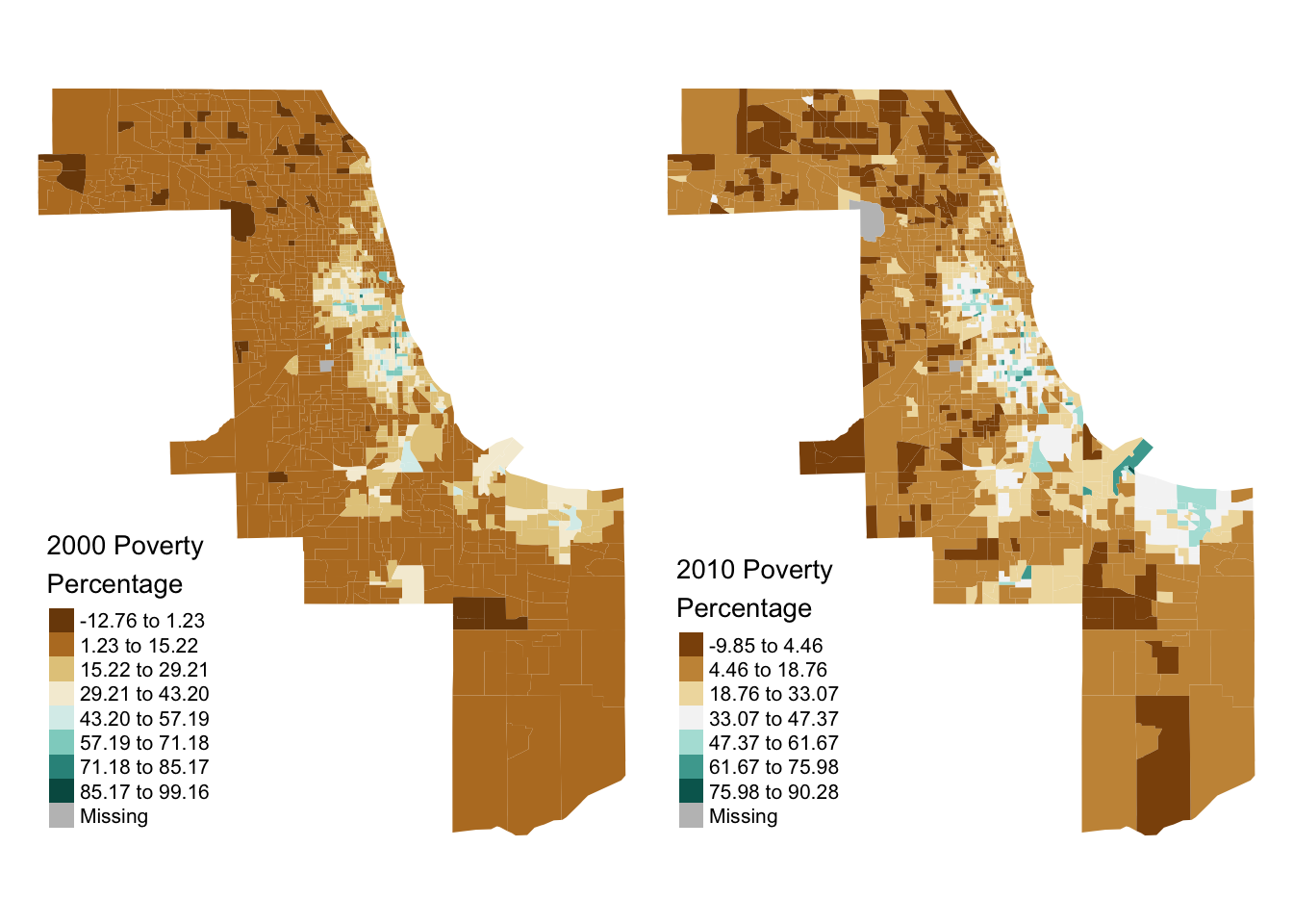
With longitudinal data in hand, we can then conduct basic analyses on our data. For instance, we can make side-by-side maps of poverty rates:
tm_shape(chicago_metro_longitudinal) +
  tm_fill(c('PovP2000', 'PovP2010'),
          title = c('2000 Poverty\nPercentage', '2010 Poverty\nPercentage'),
          style = c('sd', 'sd'),
          palette = 'BrBG') +
  tm_layout(legend.position = c('left', 'bottom'), frame=FALSE)
#>
#> ── tmap v3 code detected ───────────────────────────────────────────────────────
#> [v3->v4] `tm_fill()`: instead of `style = "sd"`, use fill.scale =
#> `tm_scale_intervals()`.
#> ℹ Migrate the argument(s) 'style', 'palette' (rename to 'values') to
#>   'tm_scale_intervals(<HERE>)'
#> For small multiples, specify a 'tm_scale_' for each multiple, and put them in a
#> list: 'fill'.scale = list(<scale1>, <scale2>, ...)'
#> [v3->v4] `tm_fill()`: migrate the argument(s) related to the legend of the
#> visual variable `fill` namely 'title' to 'fill.legend = tm_legend(<HERE>)'
#> [cols4all] color palettes: use palettes from the R package cols4all. Run
#> `cols4all::c4a_gui()` to explore them. The old palette name "BrBG" is named
#> "brewer.br_bg"
#> Multiple palettes called "br_bg" found: "brewer.br_bg", "matplotlib.br_bg". The first one, "brewer.br_bg", is returned.
#>
#> Multiple palettes called "br_bg" found: "brewer.br_bg", "matplotlib.br_bg". The first one, "brewer.br_bg", is returned.
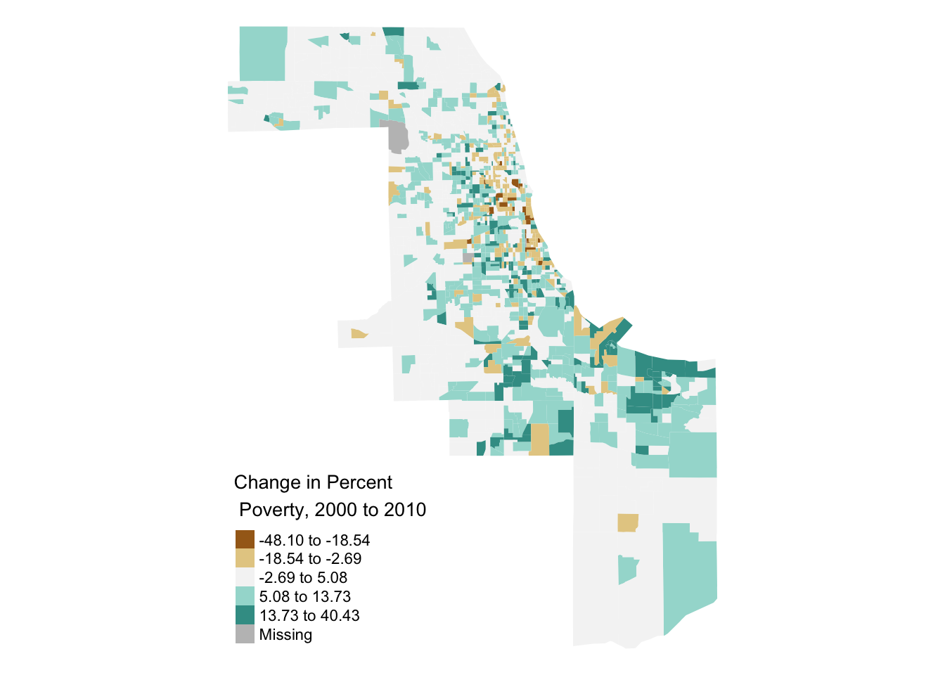
Or calculate the change in poverty:
# make a new variable
chicago_metro_longitudinal <- dplyr::mutate(chicago_metro_longitudinal,
                                       ChangePovP = PovP2010 - PovP2000)

tm_shape(chicago_metro_longitudinal) +
  tm_fill('ChangePovP',
          title = "Change in Percent\n Poverty, 2000 to 2010",
          style = 'jenks',
          palette = 'BrBG') +
  tm_layout(legend.position = c('left', 'bottom'), frame=FALSE)
#>
#> ── tmap v3 code detected ───────────────────────────────────────────────────────
#> [v3->v4] `tm_fill()`: instead of `style = "jenks"`, use fill.scale =
#> `tm_scale_intervals()`.
#> ℹ Migrate the argument(s) 'style', 'palette' (rename to 'values') to
#>   'tm_scale_intervals(<HERE>)'
#> [v3->v4] `tm_fill()`: migrate the argument(s) related to the legend of the
#> visual variable `fill` namely 'title' to 'fill.legend = tm_legend(<HERE>)'
#> [cols4all] color palettes: use palettes from the R package cols4all. Run
#> `cols4all::c4a_gui()` to explore them. The old palette name "BrBG" is named
#> "brewer.br_bg"
#> Multiple palettes called "br_bg" found: "brewer.br_bg", "matplotlib.br_bg". The first one, "brewer.br_bg", is returned.
#>
#> [scale] tm_polygons:() the data variable assigned to 'fill' contains positive and negative values, so midpoint is set to 0. Set 'midpoint = NA' in 'fill.scale = tm_scale_intervals(<HERE>)' to use all visual values (e.g. colors)
4.3 Combining outside data
In this section, we’ll demonstrate how to pair oepsData with outside data sources to glean new insights through a short case study.
Evelyn is a public policy researcher that wants to investigate the viability of two interventions to increase healthcare accessibility in her region: increased transit availability through rideshare vouchers, and increased telehealth outreach. Through a partnership with the local regional hospital, she managed to survey 110 of the hospital’s patients, getting data on how they use the facility and their access to car transit. Let’s see how the oepsData package can help Evelyn contextualize her data and create an initial hypothesis about where best to target these interventions.
Evelyn starts by using the load_oeps_dictionary command to view the variables available at the ZCTA scale. She identifies two relevant variables for her purposes: FqhcTmDr, or the drive time to the nearest Federally Qualified Healthcare Facility, and MhTmDr, or the drive time to the nearest mental health facility. Both variables are under the Environment theme, so she uses load_oeps to pull the data:
library(oepsData)
library(dplyr)
#>
#> Attaching package: 'dplyr'
#> The following objects are masked from 'package:stats':
#>
#>     filter, lag
#> The following objects are masked from 'package:base':
#>
#>     intersect, setdiff, setequal, union

zcta <- oepsData::load_oeps(scale='zcta', year='2018',
                            theme='Environment', geometry=TRUE)

zcta <- zcta[c('GEOID', 'FqhcTmDr', 'MhTmDr')]

dplyr::glimpse(zcta)
#> Rows: 32,990
#> Columns: 4
#> $ GEOID    <int> 1001, 1002, 1003, 1005, 1007, 1008, 1009, 1010, 1011, 1012, 1…
#> $ FqhcTmDr <dbl> 8.04, 0.00, 3.27, 29.70, 15.10, 18.59, 24.86, 17.61, 20.80, 1…
#> $ MhTmDr   <dbl> 8.04, 0.00, 0.00, 0.00, 15.10, 18.59, 7.56, 15.87, 34.72, 18.…
#> $ geometry <MULTIPOLYGON [°]> MULTIPOLYGON (((-72.66768 4..., MULTIPOLYGON (((…
Evelyn then filters down to the ZCTAs in her region. Depending on what data Evelyn has on hand, she has a few possible approaches. If she has a geometry for her region, she can use a spatial filter through sf:
library(sf)

# Read in data
study_region <- st_read('data/service_area.shp')
#> Reading layer `service_area' from data source
#>   `/Users/runner/work/oepsData/oepsData/data/service_area.shp'
#>   using driver `ESRI Shapefile'
#> Simple feature collection with 1 feature and 1 field
#> Geometry type: POLYGON
#> Dimension:     XY
#> Bounding box:  xmin: -79.22458 ymin: 38.20665 xmax: -78.48574 ymax: 38.8501
#> Geodetic CRS:  NAD83

# Match CRS
crs <- "EPSG:3968"
zcta <- st_transform(zcta, crs)
study_region <- st_transform(study_region, crs)

# Find ZCTAs which intersect the study region
zcta <- st_filter(zcta, study_region)
Alternatively, if she has a list of relevant ZCTAs on hand, she can directly filter on those:
# Read in list of relevant ZCTAs
relevant_zctas <- read.csv('data/zctas.csv')$x

# Filter against the relevant ZCTAs
zcta <- zcta[zcta$GEOID %in% relevant_zctas,]
Regardless of which approach she picks, her final result looks something like this:
library(tmap)
tm_shape(zcta) + tm_fill(col='FqhcTmDr', palette='Reds') + tm_borders()
#>
#> ── tmap v3 code detected ───────────────────────────────────────────────────────
#> [v3->v4] `tm_tm_polygons()`: migrate the argument(s) related to the scale of
#> the visual variable `fill` namely 'palette' (rename to 'values') to fill.scale
#> = tm_scale(<HERE>).
#> [cols4all] color palettes: use palettes from the R package cols4all. Run
#> `cols4all::c4a_gui()` to explore them. The old palette name "Reds" is named
#> "brewer.reds"
#> Multiple palettes called "reds" found: "brewer.reds", "matplotlib.reds". The first one, "brewer.reds", is returned.
With the ZCTA data in hand, Evelyn can load in her survey data and attach it.
Evelyn’s data details the home ZIP of each individual (ZCTA), whether they utilize primary care services at the local medical facility (Has_Pcp), utilize specialists at the facility (Has_Sp), receive financial aid to help cover their medical expenses (Fin_Aid), and have access to a car (Has_Car).
She’s interested in aggregate statistics, so instead of merging her data directly into the sample, she first aggregates it by ZCTA.
survey <- survey |>
  select(-RID) |>
  group_by(ZCTA) |>
  summarize(Fin_Aid   = sum(Fin_Aid), # count who receive financial aid
            Has_Pcp   = sum(Has_Pcp), # count who see a pcp
            Has_Sp    = sum(Has_Sp),  # count who see a specialist
            Has_car   = sum(Has_Car), # count with a car
            Num_Resps = n()) # count of respondents

# Full join, as not every ZCTA has a respondent
zcta <- merge(zcta, survey, by.x = "GEOID", by.y = "ZCTA", all=TRUE)
head(data.frame(zcta))
With her data merged, Evelyn starts a three step preliminary analysis. First, she checks the distribution of her responses:
tm_shape(zcta) +
  tm_fill('Num_Resps', style='cont', palette='RdPu', alpha=.8) +
  tm_borders()
#>
#> ── tmap v3 code detected ───────────────────────────────────────────────────────
#> [v3->v4] `tm_fill()`: instead of `style = "cont"`, use fill.scale =
#> `tm_scale_continuous()`.
#> ℹ Migrate the argument(s) 'palette' (rename to 'values') to
#>   'tm_scale_continuous(<HERE>)'
#> [v3->v4] `tm_fill()`: use `fill_alpha` instead of `alpha`.
#> [cols4all] color palettes: use palettes from the R package cols4all. Run
#> `cols4all::c4a_gui()` to explore them. The old palette name "RdPu" is named
#> "brewer.rd_pu"
#> Multiple palettes called "rd_pu" found: "brewer.rd_pu", "matplotlib.rd_pu". The first one, "brewer.rd_pu", is returned.
The majority of responses are from the center of her study area, near the city containing her partner medical facility, or from surrounding towns. Additionally, Evelyn doesn’t have respondents from West Virginia ZCTAs whose closest medical center is likely her partner facility.
With this info in hand, Evelyn asks an her main question: which ZCTAs would most benefit from increased transit services to and from the local Methadone Clinic and Mental Health providers, and which areas would benefit more from increased telehealth opportunities and outreach?
As a rough and tumble operationalization, she guesses that areas within a 30 minute drive of their nearest Mental Health provider and Methadone clinic but which have a below median percentage of patients with cars likely benefit most from a increased transit options, while locations further out might with fewer cars likely benefit most from increased telehealth.
To map this, she does a quick bit of data wrangling:
# What percentage of patients in a given ZCTA have cars?
zcta["Has_CarP"] <- zcta["Has_car"] / zcta["Num_Resps"] * 100
#> Warning in `[<-.data.frame`(`*tmp*`, "Has_CarP", value = structure(list(:
#> provided 2 variables to replace 1 variables
med_car_pct <- median(zcta$Has_CarP, na.rm = T)

# Which areas would benefit most from increased transit option?
zcta["More_Transit"] <- (zcta$MhTmDr <= 30) &
                          (zcta$FqhcTmDr <= 30) &
                             (zcta$Has_CarP < med_car_pct)

# Which areas would benefit most from increased telehealth?
zcta["More_Telehealth"] <- (zcta$MhTmDr > 30) &
                             (zcta$FqhcTmDr > 30) &
                              (zcta$Has_CarP < med_car_pct)

head(data.frame(zcta))
Evelyn then plots the results, highlighting the borders of the ZCTAs she believes may benefit most from increased telehealth in blue, and zctas she believe may benefit most from increased transit in red.
tm_shape(zcta) + tm_fill(col='pink', alpha=.25) +
tm_shape(filter(zcta, More_Transit)) +
  tm_fill(lwd=3, col='red') +
tm_shape(filter(zcta, More_Telehealth)) +
  tm_fill(lwd=3, col='blue') +
tm_shape(zcta) + tm_borders(lwd=.2)
#>
#> ── tmap v3 code detected ───────────────────────────────────────────────────────
#> [v3->v4] `tm_polygons()`: use `fill_alpha` instead of `alpha`.
Evelyn has thus identified six ZCTAs she thinks may benefit most from increased transit options, and one that she thinks will benefit more from increased telehealth accessibility. From here, she can and probably should continue to validate her results through multiple approaches. Computationally, she may want to check the percent of households without internet in each ZCTA – contained in the NoIntP variable she can get through another use of load_oeps – or collect increased responses to ensure her calculated percentages are accurate. Qualitatively, she may also want to validate her results against interview data from patients, to ensure that her proposed interventions agree with the needs expressed by the communities they will effect.